This is not yet a “howto”-guide, but merely some guidelines about what should be done to extract some physical data from radio observations of meteors. It is supposed that only one stream is active at a given time.
Raw counts
Generally, only the raw counts of amateur forward scatter observations are published, i.e., merely the number of echoes per time unit. This is a very poor indicator of the true meteor flux, as rates are highly modulated by the observational setup and the radiant position. When publishing raw counts or comparing counts from different set-ups, please keep this in mind.
There is a way in which raw counts over different days can be presented elegantly: by making a time-date graph, where the activity at a certain moment is indicated with a color code or something similar. An example is shown beneath. The observations are from the Prometeos setup of the University of Ghent, Belgium.
 Figure 1 – An example of a time-date graph, as recorded by the Prometeos setup of the University of Ghent, Belgium.
With such a graph, the diurnal variation of the sporadic background is immediately visible. This way of presenting raw counts is very useful for a quick determination of the observed streams or the localisation of abnormal activity.
Overdense activity
Although overdense meteors reflect the radio waves in a specular way, winds in the upper atmosphere distort the trail, often making it reflective even if is was not properly alligned initially. Overdense meteors from a given stream will thus more or less be observable over the whole part of the sky that is illuminated by the transmitter. This means the position of the radiant relative to the setup will have much less influence on the observed rates than in the underdense case, and that observations of overdense meteors will in first instance only have to be corrected for the radiant elevation, like in the visual case.
To select the overdense meteors from the observations, select only the longer echoes, say longer than 0.5 seconds (for “manual” observations, possibly all observed reflections). If you have an automated setup, select all reflections that do not have the underdense profile. Of course, beware of interference! Also try to substract the “overdense sporadic background” by looking at the number of overdense echoes at that particular time in a period with no shower activity.
The only thing to do with this reduced number of overdense meteors, is to multiply by the secans of the radiant zenith distance, like in the reduction of visual observations.
This way of reducing is supposed to yield activity profiles comparable to those obtained visually, as the same mass range is monitored. Do not use this method for radiant elevations lower than about 20 degrees.
Overdense mass distribution
The duration distribution of overdense meteors contains information about the mass index of the heavier meteoroids. To extract this, construct a cumulative log T – log N graph (where T is the duration of the meteors and N(T) is the number of meteors with durations exceeding T). Find the slope of the obtained line, primarily concentrating on the shorter echoes. This slope should be 1-s, with s the mass index. Note that the obtained mass index is the mean mass distribution of the active streams and the sporadic activity. To get the best value for the mass index, use only the data of the periods with highest stream activity, and use all the overdense meteors available. The obtained mass index of the stream will generally be a bit too large due to sporadic contamination.
Underdense activity
Underdense meteors are strictly subject to the rules of specular reflection. They are consequently only observed in the echo surface corresponding to their stream, i.e., a given strip in the sky. Rates from a given stream are only high if this echo surface is in the main lobe of the antenna. It is obvious that correcting for this geometrical selectivity is essential for getting activity information, and that a particular stream can only be observed a few hours a day with a fixed setup.
The first thing to do is to select only the underdense reflections. I guess only high speed automated systems can be used for the reliable observation of underdense meteors. When profiles were stored, select only the echoes with the typical underdense shape. When they are not, select only reflections shorter than about 0.5 s. Beware of spikes
created by electrical devices and lightning ! Try to correct for the “underdense sporadic activity” by looking at the number of underdense echoes at that time of the day in a period when no shower is active.
This “shower echo” rate can now be corrected for the geometrical selectivity described earlier. This can be done with a program like FORWARD, which
calculates the observability function given the radiant coordinates, the expected mass index of the stream, the position of the transmitter and receiver, antenna parameters, … Do not use this method when the corrections suggested by FORWARD are too large. Also note that the observability function given by FORWARD is based on many approximations, and is thus not totally reliable.
This way of reducing will generally yield activity profiles different from those obtained through visual observations, as here only the smaller particles are monitored.
Underdense mass distribution
The mass index can also be derived from an amplitude distribution. In this case, the cumulative log A – log N graph (where A is the amplitude of the meteor echo and N(A) is the number of meteoroids with amplitudes exceeding A) contains two regimes: on the left side, there is an underdense regime, where the slope is 1-s, and on the right side there is an overdense regime, where the slope is 4(1-s) in case of forward scatter and 3.57(1-s) in case of backscatter (radar). Find the slopes of the obtained lines, primarily concentrating on the lower amplitudes.
Note that, here too, the obtained mass index is the mean mass distribution of the small (underdense) or large (overdense) particles in the active streams and the sporadic activity. To get the best value for the mass index, use only the data of the periods with highest stream activity, and use all the underdense/overdense meteors available. The obtained mass index of the stream will generally be a bit too large due to sporadic contamination.
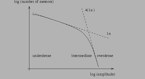 Figure 2 – The mass index can also be derived from an amplitude distribution.
General remarks
Do not use the techniques described below when the observability of the streams is too low.
Keep in mind that these methods are still very elementary. Try to correct for changes in the observational parameters, like transmitters going down at night, …
Also remember that you probably observe echoes from different transmitters. The total observability function of a stream is the sum of the observability functions for each of these transmitters.